Lab 3: Black Bear Habitats

Goal:

Lab three was designed to introduce students to working on complex geographical questions. The main premise of it was to study bears in Marquette County Michigan. With the use of GPS data and other data from the Michigan Center for Geographic Information (Supplied by Dr. Hupy) I was able to plot the bears’ locations. From this I was able to learn what their preferred habitat was, and find what parts of this habitat fell within the Michigan DNR’s territory.

This lab was divided out into 8 sections:

1.       Mapping a GPS flat file of black bear locations.

2.       Assess what type of land cover these bears prefer to spend their time.

3.       Judge whether or not streams are important when determining habitat.

4.       Map suitable bear habitat according to the above parameters.

5.       Find areas that area managed by the DNR.

6.       Exclude areas in proximity to urban areas.

7.       Build a flow model.

8.       Learn the absolute basics of python coding in ArcMap.

Objective 1:

For the first objective of the lab I was asked to take an excel file that contained locations gathered by GPS of areas which bears frequented. Seeing as it was an excel file with no object ID I was limited in how I could manipulate the data. In order to overcome the limitations of a flat file I had to define the coordinate system and import the data into ArcMap. After it was imported I compared the locations of the excel file point data with a shape file showing forest cover in my area of interest. I did this to make sure I used the correct coordinate system when importing the excel file location data. All the points fell within the study area so I was confident enough to export the excel point data into the marquette_bear_study.gdb. Exporting the data only creates a copy of the file with an object ID meaning that the attribute table can now be edited and individual points can be adjusted.

Objective 2:

Objective two is more interested in the spatial relationships between the locations of the bears and the type of land cover of the locations. Seeing as the location data for the bears only have

an ID number and coordinate data I needed to perform a simple spatial join to get land cover data included in the bear location attribute table. Figure 1 shows the results of the join. Notice the matching ID numbers for both tables and how land cover information has been added to the new bear_cover table.

Figure 1. Results of spatial table join, before (Right) and after (Left).

Now that the bears locations have been joined with the land cover type polygons I can summarize the forest type field to find out what kind of terrain bears like. Below is table that I was able to make from the combined land cover data and bear locations (Figure 2).

Figure 2. Summary table of Bears per land cover type.

From the table it is easy to tell that bears like to hang out in mixed forest land, forested wetlands, and evergreen forest land. I will need these three cover types for use later.

Objective 3:

Objective three requires me to find the percentage of bears that are within 500 meters of a stream. In order to do this I selected the bear locations according to their distance from the nearest stream. According to the lab if the percentage is above 30 then biologists consider it important for calculating bear habitat areas. According to the data 49 of 68 bears (~81.6%) were within 500 meters of a stream when their GPS locations were recorded meaning that stream locations are an important consideration when studying bear habitat. For this lab I was required to symbolize the 500 meter distance from streams. To do this I used a buffer tool to create a new dissolved polygon feature class (Figure 3) around streams. 

Figure 3. 500 meter buffer area around streams. Cyan points represent bears within 500M of a stream.

I don’t like how the stream buffer layer extends outside of the land cover polygon. Seeing as this data will probably be shown on a map and because I wanted to use a new tool, I clipped the stream buffer polygon to get it to look a little better (Figure 4). I found out later that I did not need to do this to improve the appearance of the final product but I believe the exercise was still relevant to this lab.

Figure 4. Top: map showing 500 meter buffer polygon around streams. Bottom: 500 meter buffer polygon clipped by underlying forest cover polygon.  

Objective 4:

For Objective four I was to make a Bear Habitat feature class. From the earlier objectives I learned that Bears don’t like to be too far from streams and that they love mixed forest land, forested wetlands, and evergreen forest land. These two different features are what I will use to determine the ideal bear habitat. Seeing as they are both polygons with attributes I want I used the intersect tool. See the results in the image below (Figure 5).

Figure 5. Top: intersection between a 500 meter stream buffer and forest types bears like to create suitable habitat areas. Bottom: Suitable habitat areas generalized with the buffer tool.

               

Once a suitable habitat feature was made I generalized it using a buffer tool (Figure 5). While there was some loss of information the data’s appearance was improved and still works perfectly fine for my purposes.

Objective 5:

The fifth objective had me bring in a feature class representing DNR coverage. The Michigan DNR wanted to know what areas of suitable bear habitat was within their areas of influence. In order to figure this out I used the intersect tool to preserve all areas which are within both the DNR coverage and bear habitat (Figure 6).

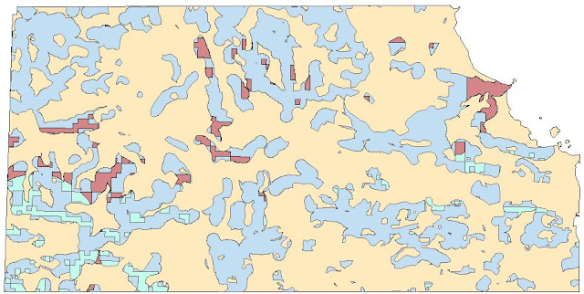
Figure 6. DNR coverage (green) within the bear habitat.

Objective 6:

The DRN are not interested in fostering an inviting habitat for bears close to developed areas in the county. So for Objective six I was required to remove the portions of the DNR bear management areas that are close to urban or built up land. So in the same fashion as I used to determine the areas bears like to visit I determined the areas they shouldn’t get to close to. I used the buffer tool to create a 5 Kilometer areas around urban areas. Once this polygon was created I could use it as an erase feature on the DNR coverage areas (Figure 7).

Figure 7. Viable areas for DNR management in red.

Objective 7:

For the seventh objective of this lab I was required to make a cartographically pleasing map and a workflow model for the entire lab. Here is what I was able to come up with:

Figure 8. Completed map of Bear Habitat study area in Marquette Michigan. 

Figure 9. Workflow Model for Figure 8.

Objective 8:

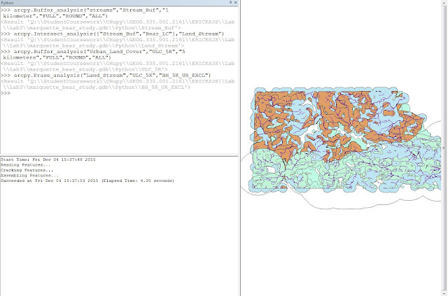
Objective eight required me to use many of the same tools as which I used earlier in the lab. There was one key change in the methods though: I was supposed to code them into ArcMap with the use of python. I have no coding experience but after a few minutes of messing around with the interface it actually turns out to be moderately easy. I was able to make a one kilometer buffer around the rivers feature class, intersect that output with the bear friendly land cover feature set, and erase any bear habitat from the display that was within five kilometers of urban areas. Below I have included a screen shot of the code and the resulting feature classes (Figure 9).

Figure 9. Python code used to create Feature Classes.